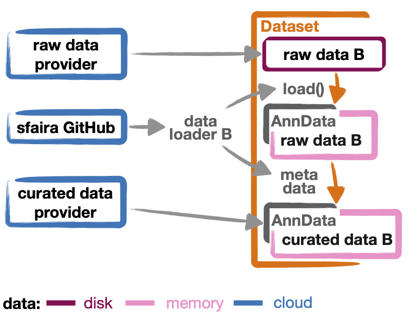
Writing data loaders
For a high-level overview of data management in sfaira, read The data life cycle first. In brief, a data loader is a set of instructions that allows for streamlining of raw count matrices and meta data into objects of a target format. Here, streamlining means that gene names are controlled based on a genome assembly, metadata items are constrained to follow ontologies, and key study metadata are described. This streamlining increases accessibility and visibility of a dataset and to makes it available to a large audience. In sfaira, data loaders are grouped by scientific study (DOI of a preprint or DOI of a publication). A data loader for a study is a directory named after the DOI of the study that contains code and text files. This directory is part of the sfaira python package and, thus, maintained on GitHub. This allows for data loaders to be maintained via GitHub workflows: contribution and fixes via pull requests and deployment via repository cloning and package installation.
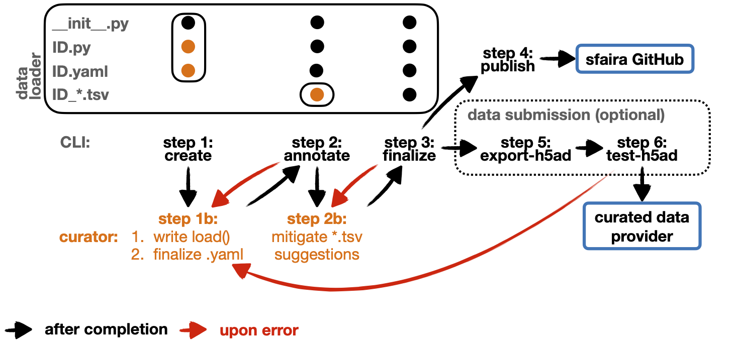
A dataloader consists of four file components within a single directory:
__init__.pyfile which is has same content in all loaders,ID.pyfile that contains aload()functions with based instructions of loading raw data on disk,ID.yamlfile that describes most meta data,ID*.tsvfiles with ontology-wise maps of free-text metadata items to constrained vocabulary.
All dataset-specific components receive an ID that is set during the curation process.
Below, we describe how multiple datasets within a study can be handled with the same dataloder.
In cases where this is not efficient, one can go through the data loader creation process once for each dataset
and then group the resulting loaders (file groups 1-4) in a single directory named after the study’s DOI.
An experienced curator can directly write such a data loader. However, first-time contributors often struggle with the interplay of individual files, metadata maps from free-text annotation are notoriously buggy and comprehensive testing is important also for contributions by experienced curators. Therefore, we broke the process of writing a loader down into phases and built a CLI to guide users through this process. Each phase corresponds to one command (one execution of a shell command) in the CLI. In addition, the CLI guides the user through manual steps that are necessary in each phase. We structured the process of curation into four phases, a preparatory phase P precedes CLI execution and is described in this documentation.
Phase P (
prepare): data and python environment setup for curation.Phase 1 (
create): aload()function (in a.py) and a YAML are written.Phase 2 (
annotate): ontology-specific maps of free-text metadata to contrained vocabulary (in*.tsv) are written.Phase 3 (
finalize): the data loader is tested and metadata are cleaned up.Phase 4 (
publish): the data loader is uploaded to the sfaira GitHub repository.
An experienced curator could skip using the CLI for phase 1 and write the __init__.py, ID.py and ID.yaml by hand.
In this case, we still highly recommend using the CLI for phase 2 and 3.
Note that phase 2 is only necessary if you have free-text metadata that needs to be mapped,
the CLI will point this out accordingly in phase 1.
This 4-phase cycle completes initial curation and results in data loader code that can be pushed to the sfaira
GitHub repository.
You have the choice between using a docker image or a sfaira installation (e.g. in conda) for phase P-4.
The workflow is more restricted but safer in conda, we recommend docker if you are inexperienced with software
development with conda, git and GitHub.
Where appropriate, separate instruction options are given for workflows in conda and docker below.
Overall, the workflow looks the same in both frameworks, though.
This cycle can be complemented by an optional workflow to cache curated .h5ad objects (e.g. on the cellxgene website):
Phase 5 (
export-h5ad): the data loader is used to create a streamlined.h5adof a particular format.Phase 6 (
validate-h5ad): the.h5adfrom phase 4 is checked for compliance with a particular (e.g. the cellxgene format).
The resulting .h5ad can be shared with collaborators or uploaded to data submission servers.
Create a new data loader
Phase P: Preparation
Before you start writing the data loader, we recommend completing this checks and preparation measures. Phase P is sub-structured into sub-phases:
- Pa. Name the data loader.
We will decide for a name of the dataloader based on its DOI. Prefix the DOI with
"d"and replace the special characters in the DOI with"_"here to prevent copy mistakes, e.g. the DOI10.1000/j.journal.2021.01.001becomesd10_1000_j_journal_2021_01_001Remember to replace this DOI with the DOI of the study you want to contribute, choose a publication (journal) DOI if available, otherwise a preprint DOI. If neither DOI is available, because this is unpublished data, for example, use an identifier that makes sense to you, that is prefixed withdno_doiand contains a name of an author of the dataset, e.g.dno_doi_einstein_brain_atlas. We will refer to this name asDOI-nameand it will be used to label the contributed code and the stored data.- Pb. Check that the data loader was not already implemented.
We will open issues for all planned data loaders, so you can search both the code base and our GitHub issues for matching data loaders before you start writing one. You can also search for GEO IDs if our code base as they are included in the data URL that is annotated in the data loader. The core data loader identified is the directory compatible doi, which is the doi with all special characters replaced by “_” and a “d” prefix is used: “10.1016/j.cell.2019.06.029” becomes “d10_1016_j_cell_2019_06_029”. Searching for this string should yield a match if it is already implemented, take care to look for both preprint and publication DOIs if both are available. We will also mention publication names in issues, you will however not find these in the code.
- Pc. Prepare an installation of sfaira to use for data loader writing.
Instead of working in your own sfaira installation, you can download the sfaira data curation docker container instead of going through any of the steps here.
- Pc-docker.
Install docker (and start Docker Desktop if you’re on Mac or Windows).
- Pull the latest version of the sfaira cli container.
sudo docker pull leanderd/sfaira-cli:latest
Run the sfaira CLI within the docker image. Please replace <path_data> and <path_loader> with paths to two empty directories on your machine. The sfaira CLI will use these to read your datafiles from and write the dataloaders to respectively.
PATH_DATA=<path_data>
PATH_LOADER=<path_loader>
sudo docker run --rm -it -v ${PATH_DATA}:/root/sfaira_data -v ${PATH_LOADER}:/root/sfaira_loader leanderd/sfaira-cli:latest
- Pc-conda.
Jump to step 4 if you do not require explanations of specific parts of the shell script.
- Install sfaira.
Clone sfaira into a local repository
DIR_SFAIRA.cd DIR_SFAIRA git clone https://github.com/theislab/sfaira.git cd sfaira git checkout dev
- Prepare a local branch of sfaira dedicated to your loader.
You can name this branch after the
DOI-name, prefix this branch withdata/as the code change suggested is a data addition.cd DIR_SFAIRA cd sfaira git checkout dev git pull git checkout -b data/DOI-name
- Install sfaira into a conda environment.
You can for example use pip inside of a conda environment dedicated to data curation.
cd DIR_SFAIRA cd sfaira git checkout -b data/DOI-name conda create -n sfaira_loader conda install -n sfaira_loader python=3.8 conda activate sfaira_loader pip install -e .
- Summary of step 1-3.
Pc1-3 are all covered by the following code block. Remember to name the git branch after your DOI:
cd DIR_SFAIRA git clone https://github.com/theislab/sfaira.git cd sfaira git checkout dev git pull git checkout -b data/DOI-name conda create -n sfaira_loader conda install -n sfaira_loader python=3.8 conda activate sfaira_loader pip install -e .
- Pd. Download the raw data into a local directory.
You will need to set a path in which the data files can be accessed by sfaira, in the following referred to as
<path_data>/<DOI-name>/. Identify the raw data files and copy them into the datafolder<path_data>/<DOI-name>/. Note that this should be the exact files that are downloadable from the download URL you provided in the dataloader: Do not decompress these files if these files are archives such as zip, tar or gz. In some cases, multiple processing forms of the raw data are available, some times even on different websites. Follow these rules to disambiguate the data source for the data loader:- Rule 1: Prefer unprocessed gene expression count data over normalised data.
Often it makes sense to provide author-normalised data in a curated object in addition to count data.
- Rule 2: Prefer dedicated data archives over websites that may be temporary
Examples of archives include EGA, GEO, zenodo, potentially temporary websites may be institute websites, cloud files linked to a person’s account.
Note that it may in exception cases make sense to collect count data and cell-wise meta data from different locations, or similar, collect normalised and count matrices from different locations. You can supply multiple data URLs below, so collect all relevant files in this phase.
- Pe. Get an overview of the published data.
Data curation is much easier if you have an idea of what the data that you are curating looks like before you start. Especially, you will notice a difference in your ability to fully leverage phase 1a if you prepare here. We recommend you load the cell-wise and gene-wise meta in a python session and explore the type of meta data provided there. You will receive further guidance throughout the curation process here, but we recommend that you try locate the following meta data items now already if they are annotated in the data set and if they are shared across the dataset or specific to a feature or observation, where the latter usually corresponds to a column in
.obsor.varof a published.h5ad, or to a corresponding column in a tabular file:single-cell assay
cell type
developmental stage
disease state
ethnicity (only relevant for human samples)
organ / tissue
organism
sex
Note that these are also the key ontology-restricted and required meta data in the cellxgene curation schema. Next, we recommend you briefly consider the available features: Are count matrices, processed matrices or spliced/unspliced RNA published? Which gene identifiers are used (symbols or ENSEMBL IDs)? Which non-RNA modalities are present in the data?
Phase 1: create
This phase creates a skeleton for a data loader: __init__.py, .py and .yaml files.
Phase 1 is sub-structured into 2 sub-phases:
1a: Create template files (
sfaira create-dataloader).1b: Completion of created files (manual).
- 1a. Create template files.
When creating a dataloader with
sfaira create-dataloaderdataloader specific attributes such as organ, organism and many more are prompted for. We provide a description of all meta data items at the bottom of this page, note that these metadata underly specific formattig and ontology constraints described below. If the requested information is not available simply hit enter to skip the entry. Note that some meta data items are always defined per data set, e.g. a DOI, whereas other meta data items may or may not be the same for all cells in a data set. For example, an entire organ may belong to one disease condition or one organ, or may consist of a pool of multiple samples that cover multiple values of the given metadata item. The questionaire and YAML are set up to guide you through finding the best fit. Note that annotating dataset-wide is preferable where possible as it results in briefer curation code. The CLI decides on anIDof this dataset within the loader that you are writing, this will be used to label all files associated with the current dataset. The CLI tells you how to continue from here, phase 1b) is always necessary, phase 2) is case-dependent and mistakes in naming the data folder in phase Pd) are flagged here. As indicated at appropriate places by the CLI, some meta data are ontology constrained. You should input symbols, ie. readable words and not IDs in these places. For example, the.yamlentryorgancould be “lung”, which is a symbol in the UBERON ontology, whereasorgan_obs_keycould be any string pointing to a column in the.obsin theanndatainstance that is output byload(), where the elements of the column are then mapped to UBERON terms in phase 2.- 1a-docker.
You can run the
create-dataloadercommand directly.sfaira create-dataloader
- 1a-conda.
In the following command, replace
DATA_DIRwith the path<path_data>/you used above. You can optionally supply--path-loadertocreate-dataloaderto change the location of the created data loader to an arbitrary directory other than the internal collection of sfaira in./sfaira/data/dataloaders/loaders/. Note: Use the default location if you want to commit and push changes from this sfaira clone.sfaira create-dataloader --path-data DATA_DIR
- 1b. Manual completion of created files (manual).
- Correct the
.yamlfile. Correct errors in
<path_loader>/<DOI-name>/ID.yamlfile and add further attributes you may have forgotten in step 2. See sec-multiple-files for short-cuts if you have multiple data sets. This step is can be skipped if there are the.yamlis complete after phase 1a). Note on lists and dictionaries in the yaml file format: Some times, you need to write a list in yaml, e.g. because you have multiple data URLs. A list looks as follows:# Single URL: download_url_data: "URL1" # Two URLs: download_url_data: - "URL1" - "URL2"
As suggested in this example, do not use lists of length 1. In contrast, you may need to map a specific
sample_fnsto a meta data in multi file loaders:sample_fns: - "FN1" - "FN2" [...] assay_sc: FN1: 10x 3' v2 FN2: 10x 3' v3
Take particular care with the usage of quotes and “:” when using maps as outlined in this example.
- Correct the
- Complete the load function.
Complete the
load()function in<path_loader>/<DOI-name>/ID.py. If you need to read compressed files directly from python, consider our guide reading-compressed-files. If you need to read R files directly from python, consider our guide reading-r-files.
Phase 2: annotate
This phase creates annotation map files: .tsv.
The metadata items that require annotation maps all non-empty entries that end on *obs_key under
dataset_or_observation_wise in the .yaml which are subject to an ontology field-descriptions:.
One file is created per such metadata ITEM, the corresponding file is <path_loader>/<DOI-name>/<ID>_<ITEM>.tsv
This means that a variable number of such files is created and dependending on the scenario, even no such files may
be necessary:
Phase 2 can be entirely skipped if no annotation maps are necessary, this is indicated by the CLI at the end of phase 1a.
Phase 2 is sub-structured into 2 sub-phases:
2a: Create metadata annotation files (
sfaira annotate-dataloader).2b: Completion of annotation (manual).
- 2a. Create metadata annotation files (
sfaira annotate-dataloader). This creates
<path_loader>/<DOI-name>/ID*.tsvfiles with meta data map suggestions for each meta data item that requires such maps. Note: You can identify the loader via--doiwith the main DOI (ie. journal > preprint if both are defined) or with the DOI-based data loader name defined by sfaira, ie.<DOI-name>in<path_loader>/<DOI-name>, which is eitherd10_*ordno_doi_*.- 2a-docker.
In the following command, replace
DOIwith the DOI of your data loader.sfaira annotate-dataloader --doi DOI
- 2a-conda.
In the following command, replace
DATA_DIRwith the path<path_data>/you used above and replaceDOIwith the DOI of your data loader. You can optionally supply--path-loadertocreate-dataloaderif the data loader is not in the internal collection of sfaira in./sfaira/data/dataloaders/loaders/.sfaira annotate-dataloader --doi DOI --path-data DATA_DIR
- 2b. Completion of annotation (manual).
Each
<path_loader>/<DOI-name>/ID*.tsvfiles contains two columns with one row for each unique free-text meta data item, e.g. each cell type label. One file is created for each*_obs_keythat requires mapping to an ontology, which are:assay_sc_obs_key,cell_line_sc_obs_key,cell_type_sc_obs_key,development_stage_sc_obs_key,disease_sc_obs_key,ethnicity_sc_obs_key,organ_sc_obs_key,organism_sc_obs_key,sex_sc_obs_key. Depending on the number of such*_obs_keyitems that are set in the.yaml, you will have between 0 amd 9.tsvfiles.- “source”:
The first column is labeled “source” and contains free-text identifiers.
- “target”:
The second column is labeled “target” and contains suggestions for matching the symbols from the corresponding ontology.
The suggestions are based on multiple search criteria, mostly on similarity of the free-text token to tokes in the ontology. Suggested tokens are separated by “:” in the target column, for each token, the same number of suggestions is supplied. We use different search strategies on each token and separate the output by strategy by “:||:”. You might notice that one strategy works well for a particular
ID*.tsvand focus your attention on that group. It is now up to you to manually mitigate the suggestions in the “target” column of each.tsvfile, for example in a text editor. Depending on the ontology and on the accuracy of the free-text annotation, these suggestions may be more or less helpful. The worst case is that you need to go to search engine of the ontology at hand for each entry to check for matches. The best case is that you know the ontology well enough to choose from the suggestions, assuming that the best match is in the suggestions. Reality lies somewhere in the middle of the two, do not be too conservative with looking items up online. We suggest to use the ontology search engine on the OLS web-interface for your manual queries. For each meta data item, the correspond ontology is listed in the detailed meta data description field-descriptions. Make sure to read our notes on cell type curation celltype-annotation.Note 1: If you compare these
ID*.tsvtotsvfiles from published data loaders, you will notice that published ones contain a third column. This column is automatically added in phase 3 if the second column was correctly filled here.Note 2: The two columns in the
ID*.tsvare separated by a tab-separator (”\t”), make sure to not accidentally delete this token. If you accidentally replace it with" ", you will receive errors in phase 3, so do a visual check after finishing your work on eachID*.tsvfile.Note 3: Perfect matches are filled wihtout further suggestions, you can often directly leave these rows as they are after a brief sanity check.
Phase 3: finalize
- 3a. Clean and test data loader.
This command will test data loading and will format the metadata maps in
ID*.tsvfiles from phase 2b). If this command passes without further change requests, the data loader is finished and ready for phase 4. Note: You can identify the loader via--doiwith the main DOI (ie. journal > preprint if both are defined) or with the DOI-based data loader name defined by sfaira, ie.<DOI-name>in<path_loader>/<DOI-name>, which is eitherd10_*ordno_doi_*.- 3a-docker.
In the following command, replace
DOIwith the DOI of your data loader.sfaira finalize-dataloader --doi DOI
- 3a-conda.
In the following command, replace
DATA_DIRwith the path<path_data>/you used above and replaceDOIwith the DOI of your data loader. You can optionally supply--path-loadertocreate-dataloaderif the data loader is not in the internal collection of sfaira in./sfaira/data/dataloaders/loaders/. Once this command passes, it will give you a message you can use in phase 4 to document this test on the pull request.sfaira finalize-dataloader --doi DOI --path-data DATA_DIR
Phase 4: publish
You will need to authenticate with GitHub during this phase.
You can push the code from with the sfaira docker with a single command or you can use git directly:
- 4a. Push data loader to the public sfaira repository.
You will test the loader one last time, this test will not throw errors if you have not introduced changes since phase 3. Note: You can identify the loader via
--doiwith the main DOI (ie. journal > preprint if both are defined) or with the DOI-based data loader name defined by sfaira, ie.<DOI-name>in<path_loader>/<DOI-name>, which is eitherd10_*ordno_doi_*.- 4a-docker.
If you are writing a data loader from within the sfaira data curation docker, you can run phase 4 with a single command. In the following command, replace
DOIwith the DOI of your data loader.sfaira test-dataloader --doi DOI sfaira publish-dataloader
You will be prompted to paste your github token in order to authenticate with github. If you do not have a token you can leave the field blank and you will be interactively guided to authenticating your github account using your browser. (You will have to manually copy a url into the browser at some point.) In certain cases you might be prompted to enter you github username and password again during the process. Please note that this requires you to enter you username and github token as before, not the password you use to log into github.com in your browser.
You will also be prompted the following by the CLI:
Where should we push the xxx branch?You generally want to select the second option here (“Create a fork of theislab/sfaira”) unless you are a member of the theislab organisation or otherwise have previously obtained write access to the sfaira repository. In this case you can select the first option (“theislab/sfaira”).- 4a-git.
You can contribute the data loader to public sfaira as code through a pull request. Note that you can also just keep the data loader in your local installation if you do not want to make it public. In the following command, replace
DATA_DIRwith the path<path_data>/you used above and replaceDOIwith the DOI of your data loader. If you have not modified any aspects of the data loader since phase 3, you can skipsfaira test-dataloaderbelow. In order to create a pullrequest you first need to fork the sfaira repository on GitHub. Once forked, you can use the code shown below to submit your new dataloader. Note: the CLI will ask you to copy a data loader testing summary into the pull request at the end of the output generated byfinalize-dataloader.sfaira test-dataloader --doi DOI --path-data DATA_DIR cd DIR_SFAIRA cd sfaira git remote set-url origin https://github.com/<user>/sfaira.git # Replace <user> with your github username. git checkout dev git add * git commit -m "Completed data loader." git push
After successfully pushing the new dataloader to your fork, you can go to github.com and create a pullrequest from your fork to the dev branch of the original sfaira repo. Please include the doi of your added dataset in the PR title
Phase 5: export-h5ad
Phase 5 and 6 are optional, see also introduction paragraphs on this documentation page.
- 5a. Export
.h5ads’s. Write streamlined dataset(s) corresponding to data loader into (an)
.h5adfile(s) according to a specific set of rules (a schema, e.g. “cellxgene”). Note: You can identify the loader via--doiwith the main DOI (ie. journal > preprint if both are defined) or with the DOI-based data loader name defined by sfaira, ie.<DOI-name>in<path_loader>/<DOI-name>, which is eitherd10_*ordno_doi_*.- 5a-docker.
In the following command, replace
DOIwith the DOI of your data loader, replaceSCHEMAwith the target data schema. You can find the resulting h5ad file in thesfaira_datadirectory you specified when starting the container. .. code-block:sfaira export-h5ad --doi DOI --schema SCHEMA --path-out /root/sfaira_data/
- 5a-conda.
In the following command, replace
DATA_DIRwith the path<path_data>/you used above, replaceDOIwith the DOI of your data loader, replaceSCHEMAwith the target data schema, and replaceOUT_DIRwith the directory to which the objects are written to. You can optionally supply--path-loadertocreate-dataloaderif the data loader is not in the internal collection of sfaira in./sfaira/data/dataloaders/loaders/. .. code-block:sfaira export-h5ad --doi DOI --path-data DATA_DIR --schema SCHEMA --path-out OUT_DIR
Phase 6: validate-h5ad
Phase 5 and 6 are optional, see also introduction paragraphs on this documentation page.
- 6a. Validate format of
.h5ad The streamlined
.h5adfiles from phase 5 are validated according to a specific set of rules (a schema).- 6a-docker.
In the following command, replace FN with the file name of the
.h5adfile to test (just the filename, not the full path here), and replaceSCHEMAwith the target data schema. The h5ad file must be placed in thesfaira_datadirectory you specified when starting the container.sfaira validate-h5ad --h5ad /root/sfaira_data/FN --schema SCHEMA
- 6a-conda.
In the following command, replace FN with ful path of the
.h5adfile to test, and replaceSCHEMAwith the target data schema. .. code-block:sfaira validate-h5ad --h5ad FN --schema SCHEMA
Advanced topics
Loading multiple files of similar structure
Only one loader has to be written for each set of files that are similarly structured which belong to one DOI.
sample_fns in dataset_structure in the .yaml indicates the presence of these files.
The identifiers listed there do not have to be the full file names.
They are received by load() as the argument sample_fn and can then be used in custom code in load() to load
the correct file.
This allows sharing code across these files in load().
If these files share all meta data in the .yaml, you do not have to change anything else here.
If a some meta data items are file specific, you can further subdefine them under the keys in this .yaml via their
identifiers stated here.
In the following example, we show how this formalism can be used to identify one file declared as “A” as a healthy
lung sample and another file “B” as a healthy pancreas sample.
dataset_structure:
    dataset_index: 1
    sample_fns:
        - "A"
        - "B"
dataset_wise:
    # ... part of yaml omitted ...
dataset_or_observation_wise:
    # ... part of yaml omitted
    healthy: True
    healthy_obs_key:
    individual:
    individual_obs_key:
    organ:
        A: "lung"
        B: "pancreas"
    organ_obs_key:
    # part of yaml omitted ...
Note that not all meta data items have to subdefined into “A” and “B” but only the ones with differing values!
The corresponding load function would be:
def load(data_dir, sample_fn, fn=None) -> anndata.AnnData:
    # The following reads either my_file_A.h5ad or my_file_B.h5ad which correspond to A and B in the yaml.
    fn = os.path.join(data_dir, f"my_file_{sample_fn}.h5ad")
    adata = anndata.read(fn)
    return adata
Loaders for meta studies or atlases
Meta studies are studies on published gene expression data.
Often, multiple previous studies are combined or meta data annotation is changed.
Data sets from such meta studies can be added to sfaira just as primary data can be added,
we ask for theses studies to be identified through the meta data attribute primary_data
to allow sfaira users to avoid duplicate cells in data universe partitions.
Let’s consider an example case:
Study A published 2 data sets A1 and A2.
Study B published 1 data set B1.
Data loaders for A and B can label as primary_data: True.
Now, study C published 1 data set C1 that consists of A2 and B1.
We can write a data loaders for C and label it as primary_data: False.
Moreover, when conducting the study C, we could even base our analyses directly on the data loaders of A2 and
B1 to make the data analysis pipeline more reproducible.
Curating cell type annotation
Common challenges in cell type curation include the following:
- An free-text label is used that is not well captured by the automated search.
Often, these are abbreviations are synonyms that can be mapped to the ontology after looking these terms up online or in the manuscript corresponding to the data loader. Indeed, it is good practice to manually verify non-trivial cell type label maps with a quick contextualization in manuscript figures or text. As for all other ontology-constrained meta data, EBI OLS maintains a great interface to the ontology under CL.
- The free-text labels contain nested annotation.
For example, a low-resolution cluster may be annotated as “T cell” in one data set, while other data sets within the same study have more specific T cell labels. Simply map each of these labels to their best fit ontology name, you do not need to mitigate differential granularity.
- The free-text labels contain cellular phenotypes that map badly to the ontology.
A common example would be “cycling cells”. In some tissues, these phenotypes can be related to specific cell types through knowledge on the phenotypes of the cell types that occur in that tissue. If this is not possible or you do not know the tissue well enough, you can leave the cell type as “UNKNOWN” and future curators may improve this annotaiton. In cases such as “cycling T cell”, you may just resort to the parent label “T cell” unless you have reason to believe that “cycling” identifies a specific T cell subset here.
- The free-text labels are more fine-grained than the ontology.
A common example would be the addition of marker gene expression to cell cluster labels that are grouped under the same ontology identifier. Some times, these marker genes can be mapped to a child node of the ontology identifier. However, often these indicate cell state variation or other, not fully attributed, variation and do not need to be accounted for in this cell type curation step. These are often among the hardest cell type curation problems, keep in mind that you want to find a reasonable translation of the existing curation, you may be limited by the ontology or by the data reported by the authors, so keep an eye on the overall effort that you spend on optimizing these label maps.
- A new cell type in annotated in free-text but is not available in the ontology yet.
This is most likely only a problem for a limited period of time in which the ontology works on adding this element. Chose the best match from the ontology and leave an issue on the sfaira GitHub describing the missing cell type. We can then later update this data loader once the ontology is updated.
Multi-modal data
Multi-modal can be represented in the sfaira curation schema, here we briefly outline what modalities are supported and how they are accounted for. You can use any combination of orthogonal meta data, e.g. organ and disease annotation, with multi-modal measurements.
- RNA:
RNA is the standard modality in sfaira, unless otherwise specified, all information in this document is centered around RNA data.
- ATAC:
We support scATAC-seq and joint scRNA+ATAC-seq (multiome) data. In both cases, the ATAC data is commonly represented as a UMI count matrix of the dimensions
(observations x peaks). Here, peaks are defined by a peak calling algorithm as part of the read processing pipeline upstream of sfaira. Peak counts can be deposited in the core data matrices managed in sfaira. The corresponding feature meta data can be set such that they allow differentiation of RNA and peak features. These features are documented dataset-or-feature-wise and feature-wise.
- protein quantification through antibody quantification:
We support CITE-seq and spatial molecular profiling assays with protein quantification read-outs. In these cases, the protein data can be represented as a gene expression matrix of the dimensions
(observations x proteins). In the case of oligo-nucleotide-tagged antibody quantification, e.g. in CITE-seq, this can also be an UMI matrix. The corresponding feature meta data can be set such that they allow differentiation of RNA and protein features. These features are documented dataset-or-feature-wise and feature-wise.
- spatial:
A couple of single-cell and spot-based assays have spatial coordinates associated with molecular profiles. We use relative coordinates of observations in a batch as
(x, y, z)tuples to characterize the spatial information. Note that spatial proximity graphs and similar spatial analyses are down-stream analyses on these coordinates. This features are documented feature-wise.
- spliced, unspliced transcript and velocities:
We support gene expression matrices on the level of spliced and unspliced transcript and the common processed format of a RNA velocity matrix. Note that the velocity matrix depends on the inference procedure. These matrices share
.varannotation with the core RNA data matrix and can, therefore, be supplemented as further layeres in theAnnDataobject without further effort. This features is documented data-matrices.
- V(D)J in TCR and BCR reconstructions:
V(D)J data is collected in parallel to RNA data in a couple of single-cell assays. We use key meta data defined by the AIRR consortium to characterize the reconstructed V(D)J genes, which are all direct outputs of V(D)J alignment pipelines and are are stored in
.obs. This features are documented feature-wise.
Reading compressed files
This is a collection of code snippets that can be used in tha load() function to read compressed download files.
See also the anndata and scanpy IO documentation.
- Read a .gz compressed .mtx (.mtx.gz):
Note that this often occurs in cellranger output for which their is a scanpy load function that applies to data of the following structure
./PREFIX_matrix.mtx.gz,./PREFIX_barcodes.tsv.gz, and./PREFIX_features.mtx.gz. This can be read as:
import scanpy
adata = scanpy.read_10x_mtx("./", prefix="PREFIX_")
- Read from within a .gz archive (.gz):
Note: this requires temporary files, so avoid if read_function can read directly from .gz.
import gzip
from tempfile import TemporaryDirectory
import shutil
# Insert the file type as a string here so that read_function recognizes the decompressed file:
uncompressed_file_type = ""
with TemporaryDirectory() as tmpdir:
    tmppth = tmpdir + f"/decompressed.{uncompressed_file_type}"
    with gzip.open(fn, "rb") as input_f, open(tmppth, "wb") as output_f:
        shutil.copyfileobj(input_f, output_f)
    x = read_function(tmppth)
- Read from within a .tar archive (.tar.gz):
It is often useful to decompress the tar archive once manually to understand its internal directory structure. Let’s assume you are interested in a file
fn_targetwithin a tar archivefn_tar, i.e. after decompressing the tar the director is<fn_tar>/<fn_target>.
import pandas
import tarfile
with tarfile.open(fn_tar) as tar:
    # Access files in archive with tar.extractfile(fn_target), e.g.
    tab = pandas.read_csv(tar.extractfile(sample_fn))
Reading R files
Some studies deposit single-cell data in R language files, e.g. .rdata, .Rds or Seurat objects.
These objects can be read with python functions in sfaira using anndata2ri and rpy2.
These modules allow you to run R code from within this python code:
def load(data_dir, **kwargs):
    import anndata2ri
    from rpy2.robjects import r
    anndata2ri.activate()

    fn = os.path.join(data_dir, "SOME_FILE.rdata")
    seurat_object_name = "tissue"
    adata = r(
        f"library(Seurat)\n"
        f"load('{fn}')\n"
        f"new_obj = CreateSeuratObject(counts = {seurat_object_name}@raw.data)\n"
        f"new_obj@meta.data = {seurat_object_name}@meta.data\n"
        f"as.SingleCellExperiment(new_obj)\n"
    )
    return adata
Loading third party annotation
In some cases, the data set in question is already in the sfaira zoo but there is alternative (third party), cell-wise
annotation of the data.
This could be different cell type annotation for example.
The underlying data (count matrix and variable names) stay the same in these cases, and often, even some cell-wise
meta data are kept and only some are added or replaced.
Therefore, these cases do not require an additional load() function.
Instead, you can contribute load_annotation_*() functions into the .py file of the corresponding study.
You can chose an arbitrary suffix for the function but ideally one that identifies the source of this additional
annotation in a human readable manner at least to someone who is familiar with this data set.
Second you need to add this function into the dictionary LOAD_ANNOTATION in the .py file, with the suffix as a key.
If this dictionary does not exist yet, you need to add it into the .py file with this function as its sole entry.
Here an example of a .py file with additional annotation:
def load(data_dir, sample_fn, **kwargs):
    pass

def load_annotation_meta_study_x(data_dir, sample_fn, **kwargs):
    # Read a tabular file indexed with the observation names used in the adata used in load().
    pass

def load_annotation_meta_study_y(data_dir, sample_fn, **kwargs):
    # Read a tabular file indexed with the observation names used in the adata used in load().
    pass

LOAD_ANNOTATION = {
    "meta_study_x": load_annotation_meta_study_x,
    "meta_study_y": load_annotation_meta_study_y,
}
The table returned by load_annotation_meta_study_x needs to be indexed with the observation names used in .adata,
the object generated in load().
If load_annotation_meta_study_x contains a subset of the observations defined in load(),
and this alternative annotation is chosen,
.adata is subsetted to these observations during loading.
You can also add functions in the .py file in the same DOI-based module in sfaira_extensions if you want to keep this
additional annotation private.
For this to work with a public data loader, you need nothing more than the .py file with this load_annotation_*()
function and the LOAD_ANNOTATION of these private functions in sfaira_extensions.
To access additional annotation during loading, use the setter functions additional_annotation_key on an instance of
either Dataset, DatasetGroup or DatasetSuperGroup to define data sets
for which you want to load additional annotation and which additional you want to load for these.
See also the docstrings of these functions for further details on how these can be set.
Required metadata
The CLI will flag any required meta data that is missing.
Note that you can use the CLI under a specific schema,
e.g. the more lenient sfaira schema (default)
or the stricter cellxgene schema, by giving the arguent --schema cellxgene to finalize-dataloader or
test-dataloader.
Moreover, .h5ad files from phase 5 can be checked for match to a particular schema in phase 6.
In brief, the following meta data are required:
dataset_structure:dataset_indexsample_fnsis required in multi-dataset loaders to define the number and identity of datasets.
dataset_wise:authorone DOI (i.e. either
doi_journalordoi_preprint)download_url_dataprimary_datayear
layers:layer_countsorlayer_processed
dataset_or_feature_wise:feature_typeorfeature_type_var_key
dataset_or_observation_wise:Either the dataset-wide item or the corresponding
_obs_keyare required to submit a data loader to sfaira:assay_scorganism
The following are encouraged in sfaira and required in the cellxgene schema:
assay_sccell_typedevelopmental_stagediseaseethnicityorganorganismsex
feature_wise:None is required.
feature_wise:feature_id_var_keyorfeature_symbol_var_key
meta:version
Field descriptions
We constrain meta data by ontologies where possible. Meta data can either be dataset-wise, observation-wise or feature-wise.
Dataset structure
Dataset structure meta data are in the section dataset_structure in the .yaml file.
- dataset_index [int]
Numeric identifier of the first loader defined by this python file. Only relevant if multiple python files for one DOI generate loaders of the same name. In these cases, this numeric index can be used to distinguish them.
- sample_fns [list of strings]
If there are multiple data files which can be covered by one
load()function and.yamlfile because they are structured similarly, these can identified here. See also sectionLoading multiple files of similar structure. You can simply hardcode a file name in theload()function and skip defining it here if you are writing a single file loader. Note: A sample is a an object similar to a count matrix or a.h5ad, the definition of biological or technical batches or samples within one count matrix does not affect this entry.
Dataset-wise
Dataset-wise meta data are in the section dataset_wise in the .yaml file.
- author [list of strings]
List of author names of dataset (not of loader).
- doi [list of strings]
DOIs associated with dataset. These can be preprints and journal publication DOIs.
- download_url_data [list of strings]
Download links for data. Full URLs of all data files such as count matrices. Note that distinct observation-wise annotation files can be supplied in download_url_meta.
- download_url_meta [list of strings]
Download links for observation-wise data. Full URLs of all observation-wise meta data files such as count matrices. This attribute is optional and not necessary ff observation-wise meta data is already in the files defined in
download_url_data, e.g. often the case for.h5ad.
- primary_data: If this is the first publication to report this gene expression data {True, False}.
This is False if the study is a meta study that uses data that was previously published. This usually implies that one can also write a data loader for the data from the primary study. Usually, the data here contains new meta data or is combined with other data sets (e.g. in an “atlas”), Therefore, this data loader is different from a data laoder for the primary data. In sfaira, we maintain data loaders both for the corresponding primary and such meta data publications. See also the section on meta studies meta-studies.
- year: Year in which sample was first described [integer]
Pre-print publication year.
Data matrices
A curated AnnData object may contain multiple data matrices: raw and processed gene expression counts, or spliced and unspliced count data and velocity estimates, for example. Minimally, you need to supply either of the matrices “counts” or “processed”. In the following, “*counts” refers to the INTEGER count of alignment events (e.g. transcripts for RNA). In the following, “*processed” refers to any processing that modifies these counts, for example: normalization, batch correction, ambient RNA correction.
layer_counts: The total event counts per feature, e.g. UMIs that align to a gene. {‘X’, ‘raw’, or a .layers key}
layer_processed: Processed complement of ‘layer_counts’. {‘X’, ‘raw’, or a .layers key}
layer_spliced_counts: The total spliced RNA counts per gene. {a .layers key}
layer_spliced_processed: Processed complement of ‘layer_spliced_counts’. {a .layers key}
layer_unspliced_counts: The total unspliced RNA counts per gene. {a .layers key}
layer_unspliced_processed: Processed complement of ‘layer_unspliced_counts’. {a .layers key}
layer_velocity: The RNA velocity estimates per gene. {a .layers key}
Dataset- or feature-wise
These meta data may be defined across the entire dataset or per feature
and are in the section dataset_or_feature_wise in the .yaml file:
They can all be supplied as NAME or as NAME_var_key:
The former indicates that the entire data set has the value stated in the yaml.
The latter, NAME_var_key, indicates that there is a column in adata.var emitted by the load() function of the name
NAME_var_key which contains the annotation per feature for this meta data item.
Note that in both cases the value, or the column values, have to fulfill constraints imposed on the meta data item as
- feature_reference and feature_reference_var_key [string]
The genome annotation release that was used to quantify the features presented here, e.g. “Homo_sapiens.GRCh38.105”. You can find all ENSEMBL gtf files on the ensembl ftp server. Here, you ll find a summary of the gtf files by release, e.g. for 105. You will find a list across organisms for this release, the target release name is the name of the gtf files that ends on
.RELEASE.gtf.gzunder the corresponding organism. For homo_sapiens and release 105, this yields the following reference name “Homo_sapiens.GRCh38.105”.
- feature_type and feature_type_var_key {“rna”, “protein”, “peak”}
The type of a feature:
- “rna”: gene expression quantification on the level of RNA
e.g. from scRNA-seq or spatial RNA capture experiments
- “protein”: gene expression quantification on the level of proteins
e.g. via antibody counts in CITE-seq or spatial protocols
- “peak”: chromatin accessibility by peak
e.g. from scATAC-seq
Dataset- or observation-wise
These meta data may be defined across the entire dataset or per observation
and are in the section dataset_or_observation_wise in the .yaml file:
They can all be supplied as NAME or as NAME_obs_key:
The former indicates that the entire data set has the value stated in the yaml.
The latter, NAME_obs_key, indicates that there is a column in adata.obs emitted by the load() function of the name
NAME_obs_key which contains the annotation per observation for this meta data item.
Note that in both cases the value, or the column values, have to fulfill constraints imposed on the meta data item as
outlined below.
- assay_sc and assay_sc_obs_key [ontology term]
The EFO label corresponding to single-cell assay of the sample. The corresponding subset of EFO_SUBSET is the set of child nodes of “single cell library construction” (EFO:0010183).
- assay_differentiation and assay_differentiation_obs_key [string]
Try to provide a base differentiation protocol (eg. “Lancaster, 2014”) as well as any amendments to the original protocol.
- assay_type_differentiation and assay_type_differentiation_obs_key {“guided”, “unguided”}
For cell-culture samples: Whether a guided (patterned) differentiation protocol was used in the experiment.
- bio_sample and bio_sample_obs_key [string]
Column name in
adata.obsemitted by theload()function which reflects biologically distinct samples, either different in condition or biological replicates, as a categorical variable. The values of this column are not constrained and can be arbitrary identifiers of observation groups. You can concatenate multiple columns to build more fine grained observation groupings by concatenating the column keys with*in this string, e.g.patient*treatmentto get onebio_samplefor each patient and treatment. Note that the notion of biologically distinct sample is slightly subjective, we allow this element to allow researchers to distinguish technical and biological replicates within one study for example. See also the meta data itemsindividualandtech_sample.
- cell_line and cell_line_obs_key [ontology term]
Cell line name from the cellosaurus cell line database.
- cell_type and cell_type_obs_key [ontology term]
Cell type name from the Cell Ontology CL database. Note that sometimes, original (free-text) cell type annotation is provided at different granularities. We recommend choosing the most fine-grained annotation here so that future re-annotation of the cell types in this loader is easier. You may choose to compromise the potential for re-annotation of the data loader with the size of the mapping
.tsvthat is generated during annotation: This file has one row for free text label and may be undesirably large in some cases, which reduces accessibilty of the data loader code for future curators, thus presenting a trade-off. See also the section on cell type annotation celltype-annotation.
- disease and disease_obs_key [ontology term]
Choose from MONDO.
- ethnicity and ethnicity_obs_key [ontology term]
Choose from HANCESTRO.
- gm and gm_obs_key [string]
Genetic modification. E.g. identify gene knock-outs or over-expression as a boolean indicator per cell or as guide RNA counts in approaches like CROP-seq or PERTURB-seq.
- individual and individual_obs_key [string]
Column name in
adata.obsemitted by theload()function which reflects the indvidual sampled as a categorical variable. The values of this column are not constrained and can be arbitrary identifiers of observation groups. You can concatenate multiple columns to build more fine grained observation groupings by concatenating the column keys with*in this string, e.g.group1*group2to get oneindividualfor each group1 and group2 entry. Note that the notion of individuals is slightly mal-defined in some cases, we allow this element to allow researchers to distinguish sample groups that originate from biological material with distinct genotypes. See also the meta data itemsindividualandtech_sample.
- organ and organ_obs_key [ontology term]
The UBERON label of the sample. This meta data item ontology is for tissue or organ identifiers from UBERON.
- organism and organism_obs_key. [ontology term]
The NCBItaxon label of the main organism sampled here. For a data matrix of an infection sample aligned against a human and virus joint reference genome, this would “Homo sapiens” as it is the “main organism” in this case. For example, “Homo sapiens” or “Mus musculus”. See also the documentation of feature_reference to see which orgainsms are supported.
- primary_data [bool]
Whether contains cells that were measured in this study (ie this is not a meta study on published data).
- sample_source and sample_source_obs_key. {“primary_tissue”, “2d_culture”, “3d_culture”, “tumor”}
Which cellular system the sample was derived from.
- sex and sex_obs_key. Sex of individual sampled. [ontology term]
The PATO label corresponding to sex of the sample. The corresponding subset of PATO_SUBSET is the set of child nodes of “phenotypic sex” (PATO:0001894).
- source_doi and source_doi_obs_key [string]
If this dataset is not primary data, you can supply the source of the analyzed data as a DOI per dataset or per cell in this meta data item. The value of this metadata item (or the entries in the corresponding
.obscolumn) needs to be a DOI
- state_exact and state_exact_obs_key [string]
Free text description of condition. If you give treatment concentrations, intervals or similar measurements use square brackets around the quantity and use units:
[1g]
- tech_sample and tech_sample_obs_key [string]
Column name in
adata.obsemitted by theload()function which reflects technically distinct samples, either different in condition or technical replicates, as a categorical variable. Any data batch is atech_sample. The values of this column are not constrained and can be arbitrary identifiers of observation groups. You can concatenate multiple columns to build more fine grained observation groupings by concatenating the column keys with*in this string, e.g.patient*treatment*protocolto get onetech_samplefor each patient, treatment and measurement protocol. See also the meta data itemsindividualandtech_sample.
- treatment and treatment_obs_key [string]
Treatment of sample, e.g. compound names in stimulation experiments.
Feature-wise
These meta data are always defined per feature and are in the section feature_wise in the .yaml file:
- feature_id_var_key [string]
Name of the column in
adata.varemitted by theload()which contains ENSEMBL gene IDs. This can also be “index” if the ENSEMBL gene names are in the index of theadata.vardata frame. Note that you do not have to map IDs to a specific annotation release but can keep them in their original form. If available, IDs are preferred over symbols.
- feature_symbol_var_key [string]
Name of the column in
adata.varemitted by theload()which contains gene symbol: HGNC for human and MGI for mouse. This can also be “index” if the gene symbol are in the index of theadata.vardata frame. Note that you do not have to map symbols to a specific annotation release but can keep them in their original form.
Observation-wise
These meta data are always defined per observation and are in the section observation_wise in the .yaml file:
The following items are only relevant for spatially resolved data, e.g. spot transcriptomics or MERFISH:
- spatial_x_coord, spatial_y_coord, spatial_z_coord [string]
Spatial coordinates (numeric) of observations. Most commonly, the centre of a segment or of a spot is indicated here. For 2D data, a z-coordinate is not relevant and can be skipped.
The following items are only relevant for V(D)J reconstruction data, e.g. TCR or BCR sequencing in single cells.
These meta data items are described in the AIRR project, search the this link for the element in question without
the prefixed “vdj_”.
These 10 meta data items describe chains (or loci).
In accordance with the corresponding scirpy defaults, we allow for up to two loci per cell.
In T cells, this correspond to two VJ loci (TRA) and two VDJ loci (TRB).
You can set the prefix of the column of each of the four loci below.
In total, these 10+4 meta data queries in sfaira describe 4*10 columns in .obs after .load().
Note that for this to work, you need to stick to the naming convention PREFIX_SUFFIX.
We recommend that you use scirpy.io functions for reading the VDJ data in your load()
to use the default meta data keys suggested by the CLI and to guarantee that this naming convention is obeyed.
- vdj_vj_1_obs_key_prefix
Prefix of key of columns corresponding to first VJ gene.
- vdj_vj_2_obs_key_prefix
Prefix of key of columns corresponding to second VJ gene.
- vdj_vdj_1_obs_key_prefix
Prefix of key of columns corresponding to first VDJ gene.
- vdj_vdj_2_obs_key_prefix
Prefix of key of columns corresponding to second VDJ gene.
- vdj_c_call_obs_key_suffix
Suffix of key of columns corresponding to C gene.
- vdj_consensus_count_obs_key_suffix
Suffix of key of columns corresponding to number of reads contributing to consensus.
- vdj_d_call_obs_key_suffix
Suffix of key of columns corresponding to D gene.
- vdj_duplicate_count_obs_key_suffix
Suffix of key of columns corresponding to number of duplicate UMIs.
- vdj_j_call_obs_key_suffix
Suffix of key of columns corresponding to J gene.
- vdj_junction_obs_key_suffix
Suffix of key of columns corresponding to junction nt sequence.
- vdj_junction_aa_obs_key_suffix
Suffix of key of columns corresponding to junction aa sequence.
- vdj_locus_obs_key_suffix
Suffix of key of columns corresponding to gene locus, i.e IGH, IGK, or IGL for BCR data and TRA, TRB, TRD, or TRG for TCR data.
- vdj_productive_obs_key_suffix
Suffix of key of columns corresponding to locus productivity: whether the V(D)J gene is productive.
- vdj_v_call_obs_key_suffix
Suffix of key of columns corresponding to V gene.
Meta
These meta data contain information about the curation process and schema:
- version: [string]
Version identifier of meta data scheme.